R - meta programmation | neonira’s blog

Lately, R meta programmation seems to be in vogue. Very huge promises, encompassing code to produce code, variable indirection naming schemes, and many others marvelous features are now available through the tidyverse. Indeed, very huge promises, are generally the right sensor to enter into skepticism and to verify by our-self it worth or not to switch from well-known and limited code approaches, to less-known more promising and more modern code approaches

A simple use case

To start small, I just used meta programmation for a very simple case, that is access to data embedded into a data.table, using various variable kind of parameters.

Two main requirements are

parameter number is not known in advanced,
parameter might be given as string or symbol.

Implementation

First approach: rely solely on data.table capabilities, using strings

filter_by_string_builtin <- function(dt, ...) {
  dt[, ..., with = FALSE]
} 

Here, the limit is that you can not pass symbols in the call. You must use strings.

Second approach: rely solely on data.table capabilities, using symbols

filter_by_symbol_builtin <- function(dt, ...) {
  dt[, ...]
}

Here, the limit is that you can pass only symbols in the call. You must not use strings.

Third approach: use data.table capabilities and meta-programmation

filter_by_symbol <- function(dt, ...) {
  sy <- ensyms(...)
  ss <- sapply(sy, as_string)
  dt[, ss, with = FALSE]
}

Here you may use strings or symbols, or even mix them.

Fourth approach: use tidyverse

filter_by_quosure <- function(dt, ...) {
  sy <- enquos(...)
  #if (length(sy) == 0) return(dt)
  dt %>%
    select(!!!sy)
}

Here you may use strings or symbols, or even mix them.

Run it by hand

All of them provide right (from a functional point of view) and identical answer. OK, but what about performance ?

mm <- microbenchmark(filter_by_string_builtin(dt, 'x', 'r'),
                     filter_by_symbol_builtin(dt, x, r),
                     filter_by_symbol(dt, 'x', 'r'),
                     filter_by_symbol(dt, x, r),
                     filter_by_quosure(dt, 'x', 'r'),
                     filter_by_quosure(dt, x, r),
                     times = 1000
)

dz <- summary(mm)
dk <- as.data.table(tidyr::gather(dz, what, data, min:max))
dk[, `:=`(x = rep(1:6, 6), what = factor(what, levels = unique(dk$what), ordered = TRUE))]
g <- ggplot(dk, aes(x = what, y = data, group = expr, color = expr)) + 
  geom_line(size = 2) +
  ggtitle(paste0('Microbenchmark - 6 number timing (', dk[1]$neval, ' evaluations)')) + 
  theme(legend.position = 'top')

h <- ggplot(dk[what != 'max'], aes(x = what, y = data, group = expr, color = expr)) + 
  geom_line(size = 2) +
  ggtitle(paste0('Microbenchmark - 5 number timing (', dk[1]$neval, ' evaluations)')) + 
  theme(legend.position = 'top')

sf <- function(e) e / e[1]
dk[, `:=`(p = sf(data)), by = 'what']

p <- ggplot(dk[what != 'max'], aes(x = what, y = p, group = expr, color = expr)) + 
  geom_line(size = 2) +
  ggtitle(paste0('Microbenchmark - 5 number timing ratio (', dk[1]$neval, ' evaluations)')) + 
  ylab('ratio in comparison to best performing approach') + xlab('') + 
  theme(legend.position = 'top')

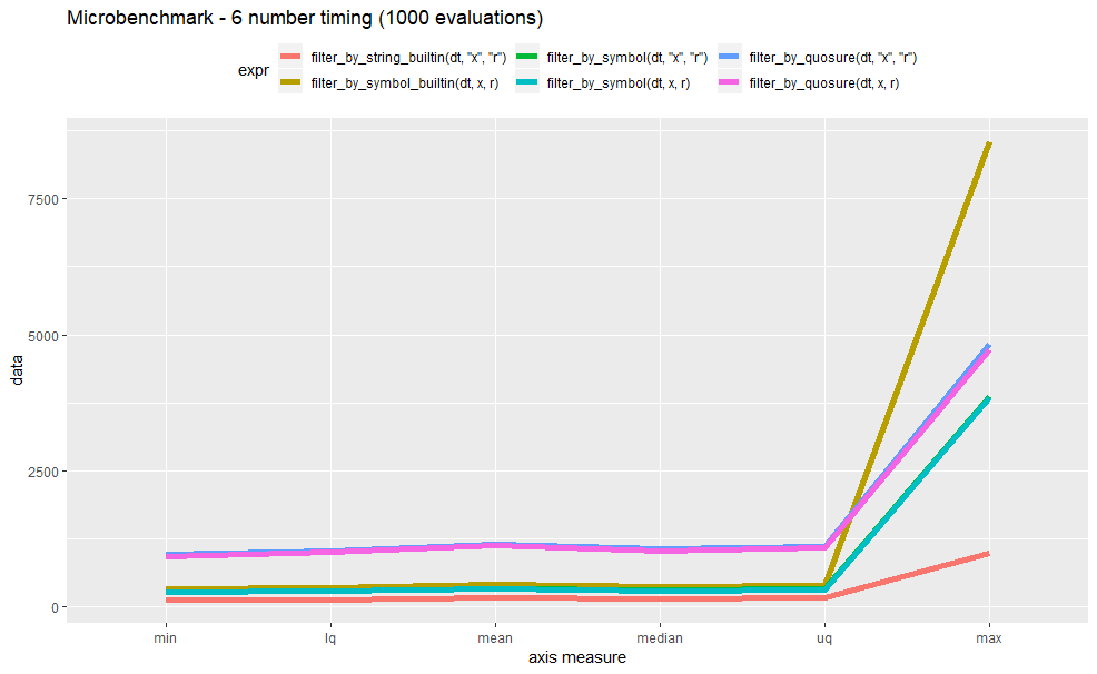
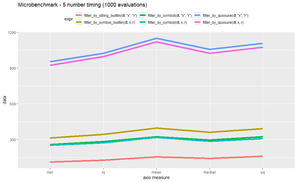
And performance data are

Unit: microseconds
                                   expr   min      lq      mean  median      uq    max neval
 filter_by_string_builtin(dt, "x", "r") 111.1  128.20  154.0355  141.90  158.95  978.2  1000
     filter_by_symbol_builtin(dt, x, r) 314.2  342.50  395.2979  360.40  392.30 8550.7  1000
         filter_by_symbol(dt, "x", "r") 258.8  282.00  324.2122  295.70  324.55 3856.1  1000
             filter_by_symbol(dt, x, r) 252.4  274.10  318.1286  285.90  309.30 3847.1  1000
        filter_by_quosure(dt, "x", "r") 953.8 1023.80 1149.2981 1055.25 1107.05 4817.4  1000
            filter_by_quosure(dt, x, r) 922.6  995.25 1118.5169 1024.50 1074.30 4728.6  10003

Some graphs to ease comparisons

global comparisons

main comparisons

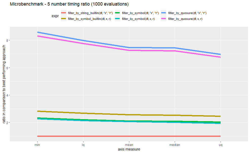
relative performance comparisons

Test context

All tests are executed disconnected from any network, on the same machine, at the same time. More information below, about hardware used, capabilities, and software versions used.

$session
R version 3.5.2 (2018-12-20)
Platform: x86_64-w64-mingw32/x64 (64-bit)
Running under: Windows >= 8 x64 (build 9200)

Matrix products: default

locale:
[1] LC_COLLATE=French_France.1252  LC_CTYPE=French_France.1252    LC_MONETARY=French_France.1252
[4] LC_NUMERIC=C                   LC_TIME=French_France.1252    

attached base packages:
[1] stats     graphics  grDevices utils     datasets  methods   base     

other attached packages:
 [1] ggplot2_3.1.0        microbenchmark_1.4-6 dplyr_0.7.8          lobstr_1.0.1         Rcpp_1.0.0          
 [6] crayon_1.3.4         rlang_0.3.1          purrr_0.2.5          data.table_1.11.8    lubridate_1.7.4     
[11] stringr_1.3.1       

loaded via a namespace (and not attached):
 [1] pillar_1.3.1     compiler_3.5.2   plyr_1.8.4       bindr_0.1.1      tools_3.5.2      digest_0.6.18   
 [7] evaluate_0.12    tibble_2.0.1     gtable_0.2.0     pkgconfig_2.0.2  rstudioapi_0.9.0 yaml_2.2.0      
[13] xfun_0.4         bindrcpp_0.2.2   knitr_1.21       withr_2.1.2      grid_3.5.2       tidyselect_0.2.5
[19] glue_1.3.0       R6_2.3.0         rmarkdown_1.11   tidyr_0.8.2      magrittr_1.5     scales_1.0.0    
[25] htmltools_0.3.6  assertthat_0.2.0 colorspace_1.4-0 labeling_0.3     stringi_1.2.4    lazyeval_0.2.1  
[31] munsell_0.5.0   

$hardware
$hardware$os
[1] "Microsoft Windows 10 Professionnel"

$hardware$os_version
[1] "10.0.17134 Number 17134"

$hardware$hardware
[1] "HP ZBook Studio G4"

$hardware$processor
[1] "Intel(R) Core(TM) i7-7820HQ CPU @ 2.90GHz, 2904MHz, 4 coeurs, 8 processeurs logiques"

$hardware$ram
[1] "16Gb"

Conclusion

On this example, it is very clear that meta-programmation has a performance cost. Minimal cost ratio of using symbols instead of strings is above 1.6, in all cases I studied. Remarkably, filter_by_symbol_builtin performs worst than filter_by_symbol. Using quosures seems to bring a huge overhead as performance ratio exceeds 5. This implementation, although quite straight and simple, might not be optimal (your suggestions are welcome).

Knowing that implementation time of the various approaches requires quite different time and concentration efforts, we may really consider when is it worth to use meta-programmation.

As a rule of thumb, here is my empirical approach

stick to existing features, using non standard evaluation schemes provided as a standard. Reuse them as is. This applies to data.table, ggplot2 packages and to other packages provinding such features.
prefer string arguments over symbol arguments wherever and whenever possible, as it simplifies inception and seems to drain better performance from current packages implementation.
restrain from using meta-programmation at a wide-scale. Keep it for clear and really useful use cases. Ease of maintenance and code volume reduction are wrong arguments here. R is based upon functions and functional programming, use it priorly to meta-programmation.

I had several tries in very different situations with meta-programming and I am still not fully convinced. Until now, I understand and feel the cost in inception and performance, but I do not perceive real value beyond promises. Some may argue about how easy is to handle data using dplyr. I would say not as easy as directly handling data.table (especially if you know this package well). Some would tell that tidyverse is the right way. It might. I like ggplot2, tidyr, rmarkdown and some other packages from it. I am fond of tidy data approach, but still remain suspicious about meta-programmation. My various real-life experience have not identified or proven any case yet, really in favor of meta-programmation. Just wondering if I haven’t miss a key about it ?